
First, this was our final project for Physics 223 here at South Seattle College. A last ditch effort to pull off something PHYSICALLY AMAZING before the end of the quarter and culmination of the Engineering Physics series. With not much time to pull it off, a Hail Mary felt accurate.
Second, the Andy Weir novel was everywhere at the time with the release of the movie adaptation starring Ryan Gosling. In the story, a microorganism called Astrophage is literally eating the sun's energy output, slowly dimming it and threatening all life on Earth. The whole plot is one desperate mission to stop it.
Our experiment is kind of the mirror image of that: instead of something consuming the sun's energy as a threat, we're studying how a solar panel harvests that energy. How it "eats" sunlight and turns it into power. Same sun. Opposite problem. And the poster was too good not to use. We replaced Gosling's name with ours. He'll be fine.
How does incident angle and shading affect electrical power output of a solar panel, and which factor has a greater impact on efficiency?
We guessed that the relationship would be linear for each factor.
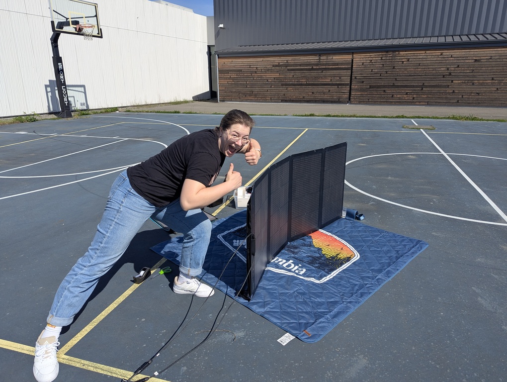
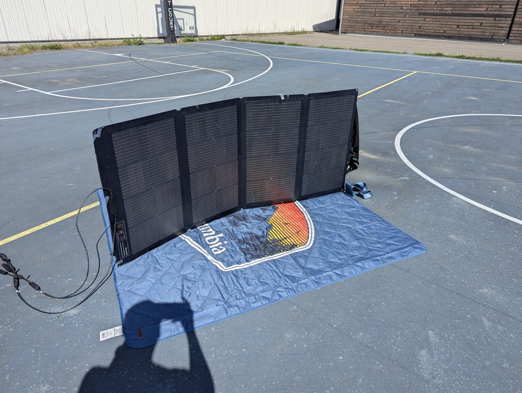
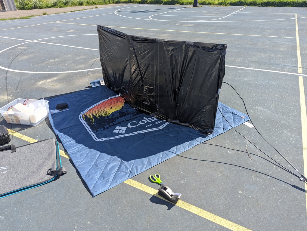
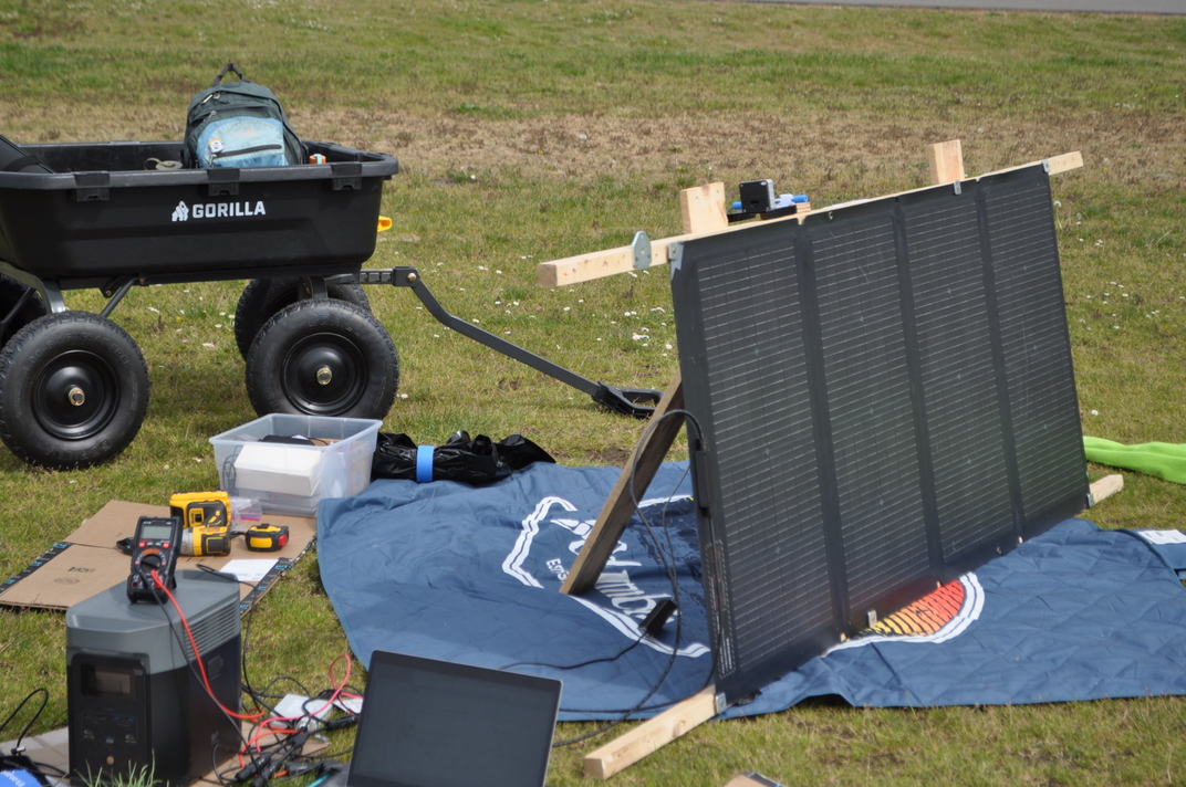
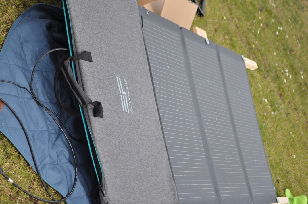
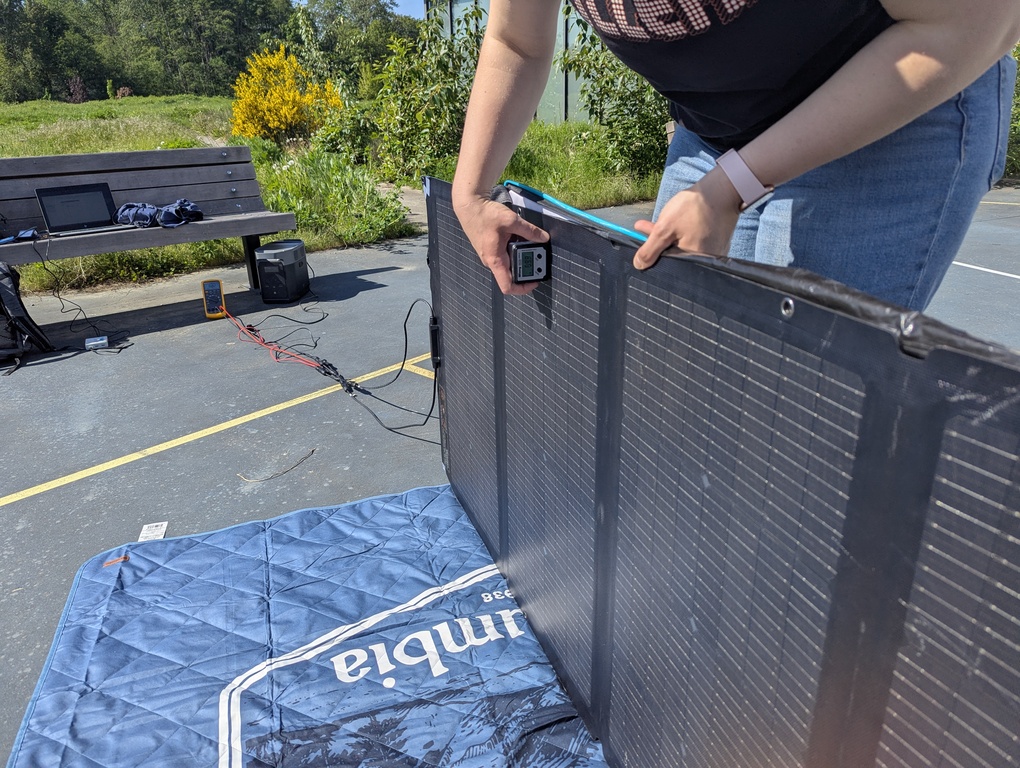
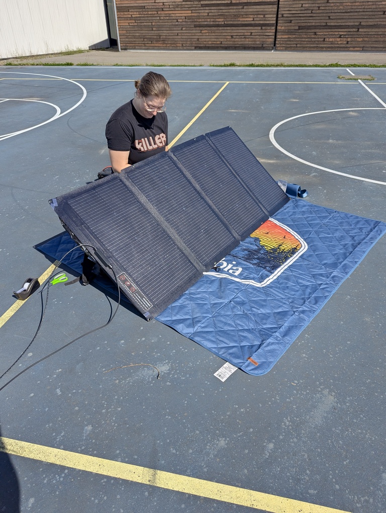
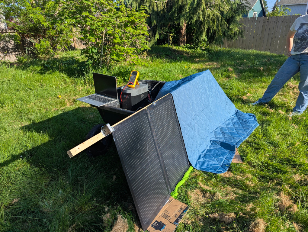
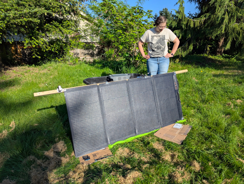
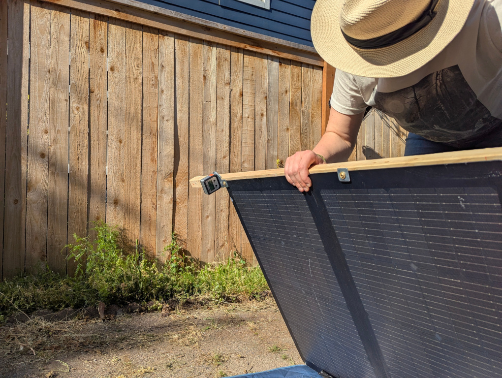
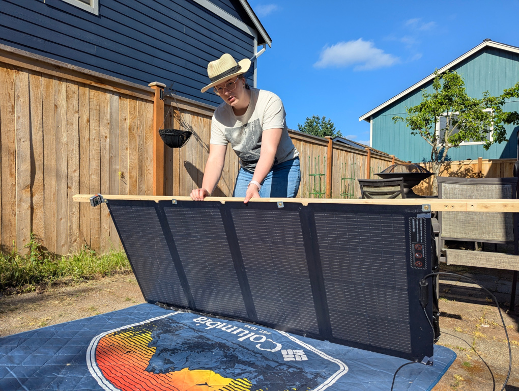
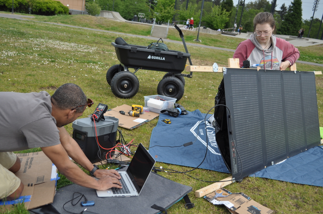
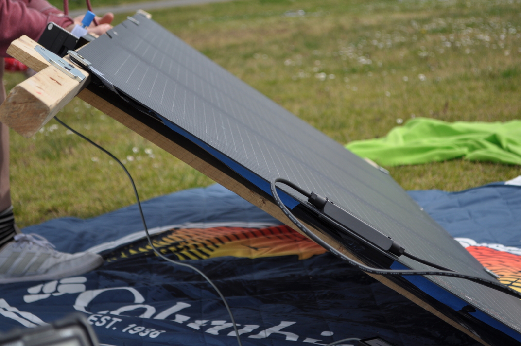
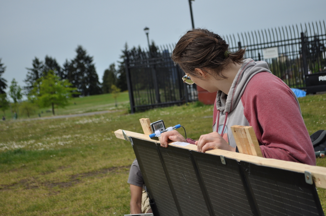
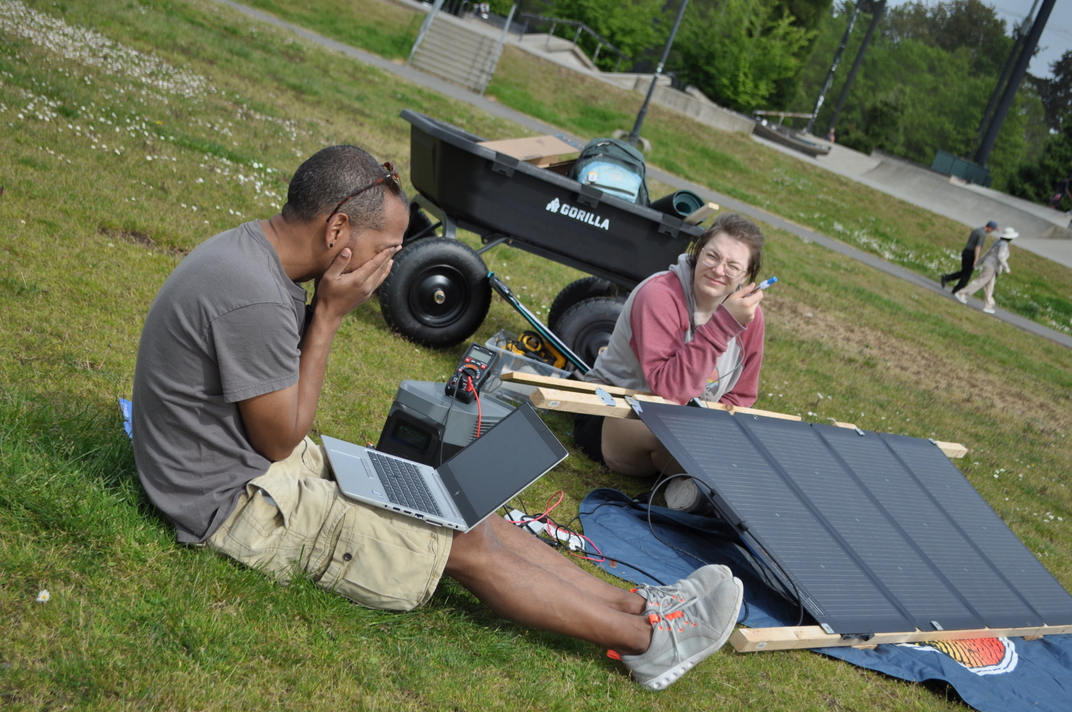
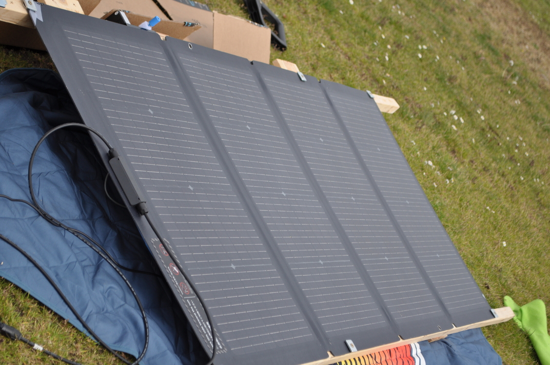
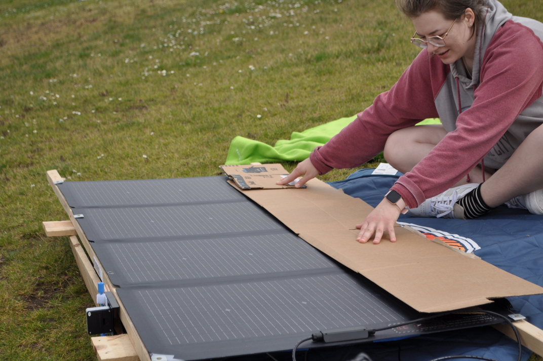
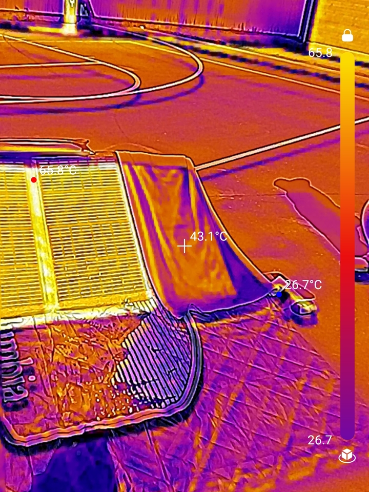
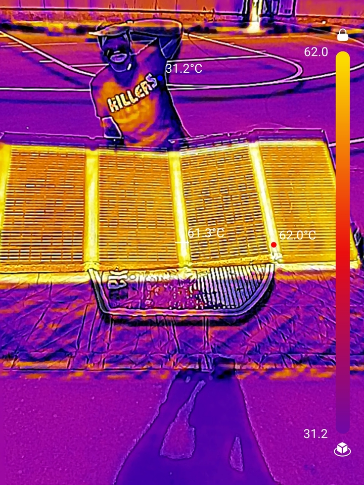
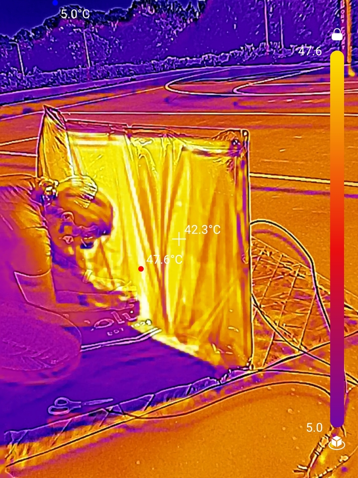
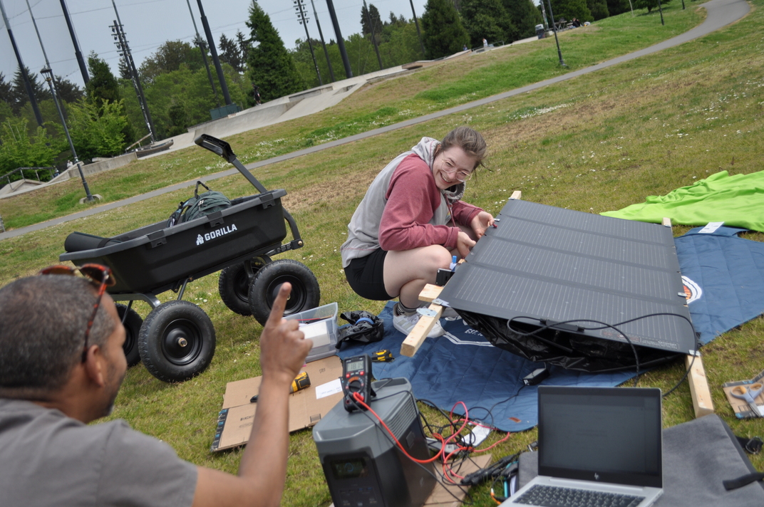
We took an EcoFlow EF-Flex-220B panel (220W rated, ~180W in real-world conditions), took it outside, pointed it at the sun, and rotated it away in measured steps while recording power output. Worth noting: the panel is bifacial, meaning it has photovoltaic cells on both sides. To keep our readings clean we covered the back side so only the front was generating power. We collected data on three different days, first angling the solar panel at regular intervals, then blocking off sub-panels and taking power readings at each stage.
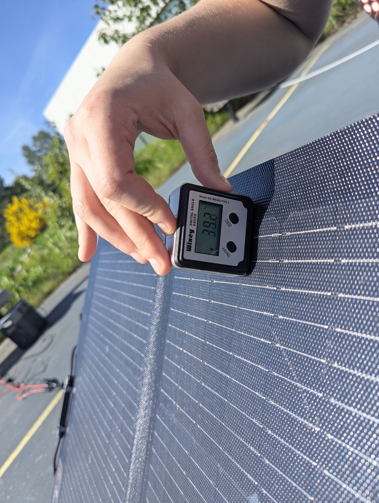
We defined 0° incident angle empirically: wherever the panel read its highest power output, that was our reference zero. From there we rotated outward and logged what happened. No prior assumptions about what the curve should look like. Just find max power, call it zero, go from there.
When we plotted the data, the curve had a clear shape to it. We fit a 2nd-degree polynomial to it, which tracked our measurements well. Then we started digging into why the curve looked the way it did, and that's when we came across Lambert's cosine law and the concept of Lambertian surfaces. Turns out there's a whole body of physics that describes exactly what we were seeing. We hadn't set out to test it. We just found it along the way.
EcoFlow EF-Flex-220B: monocrystalline silicon, 220W rated at STC, about 180W in real-world conditions. Internally it has 4 sub-panels wired in parallel, with the photovoltaic cells inside each sub-panel wired in series. That parallel/series combo matters more than it sounds (see the Observations section).
Not sure what these mean? Check out the Specs & Glossary section.
- EcoFlow EF-Flex-220B: the panel itself
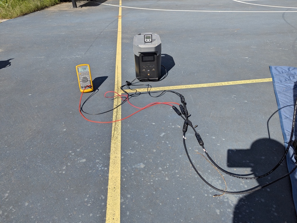
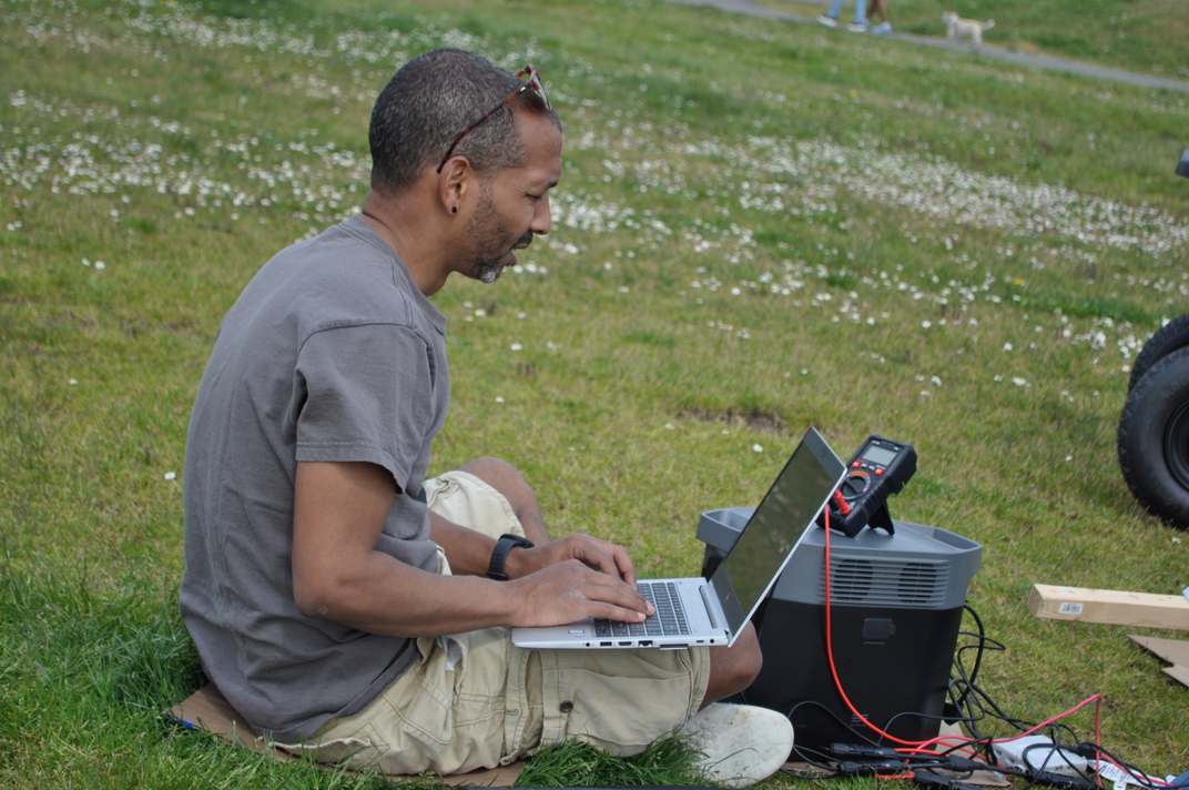
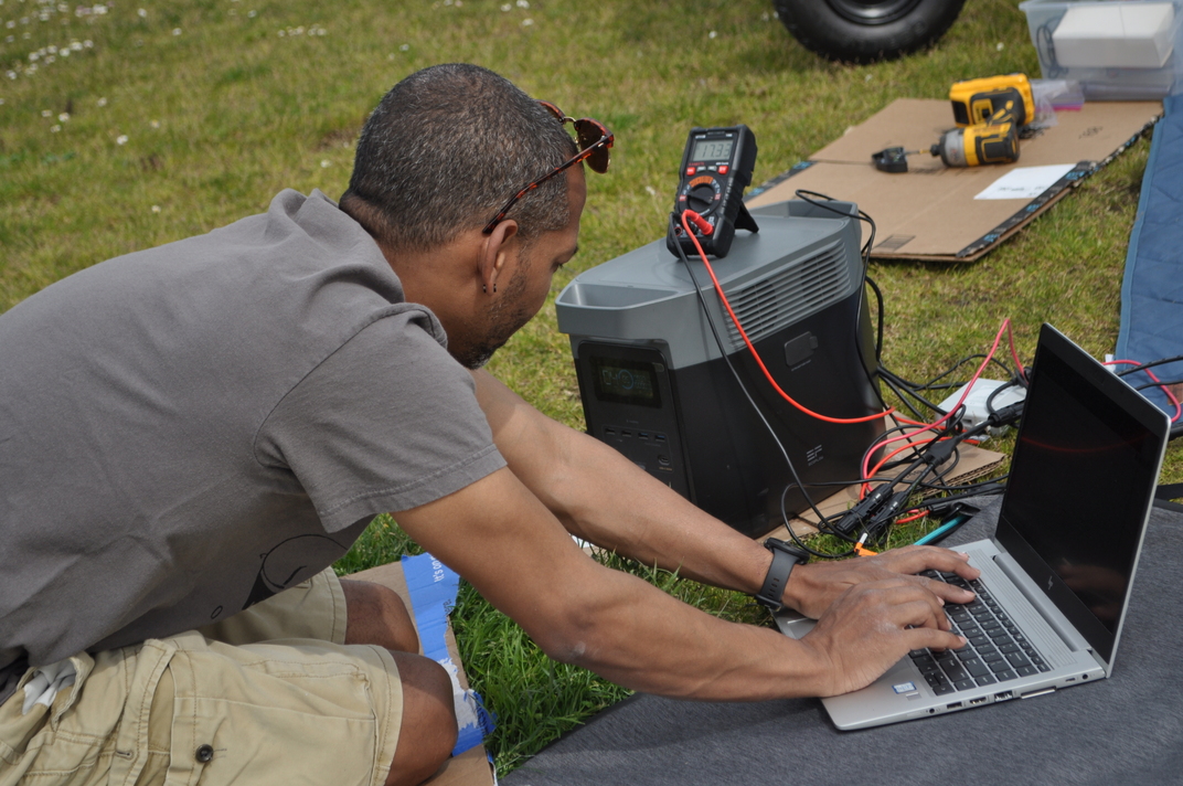
- EcoFlow DELTA 2 Max Portable Power Station: load and power measurement
- Digital Multimeter: voltage verification
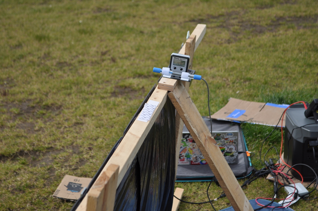
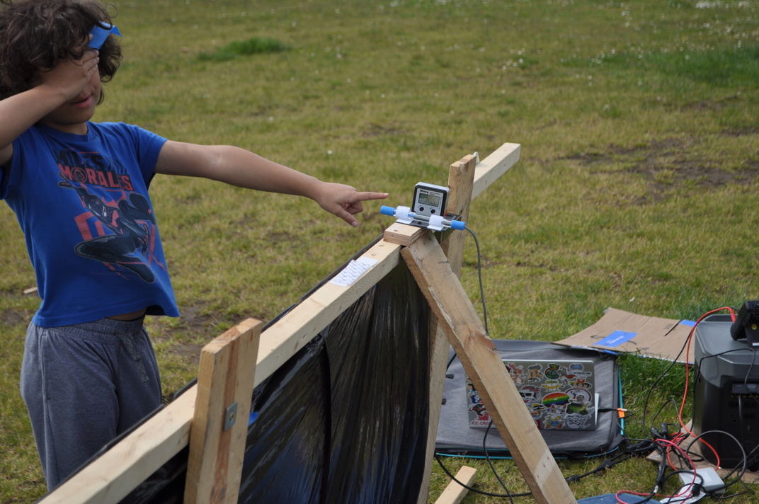
- Wixey Digital Angle Gauge: for precise incident angle measurement
- Vernier LabQuest Mini + Lux Meter: light intensity logging
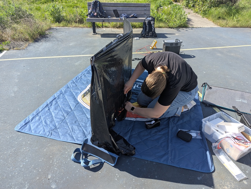
- Columbia Outdoor Blanket from Costco, cardboard, and 3 fingers: panel blockers for the shading experiment (we used what was nearby)
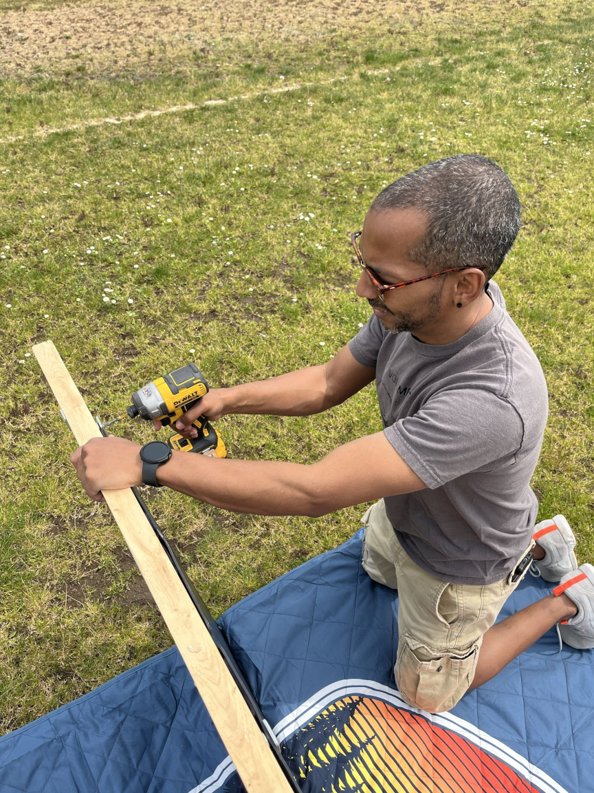
- Custom wooden frame: built to stabilize the panel at various angles
- A drill, some screws and washers, and a lot of sweat: for building said frame
- Digital camera + a minor who earned $5 taking pictures: documentation crew
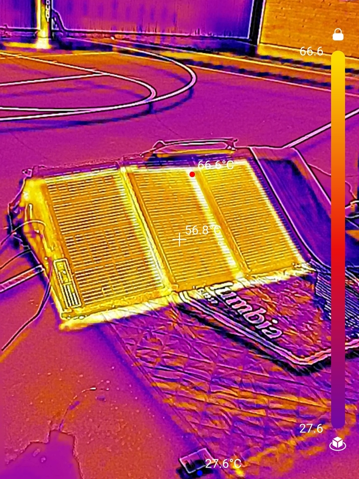
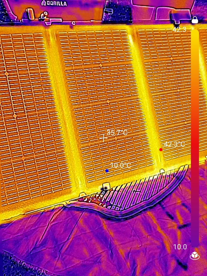
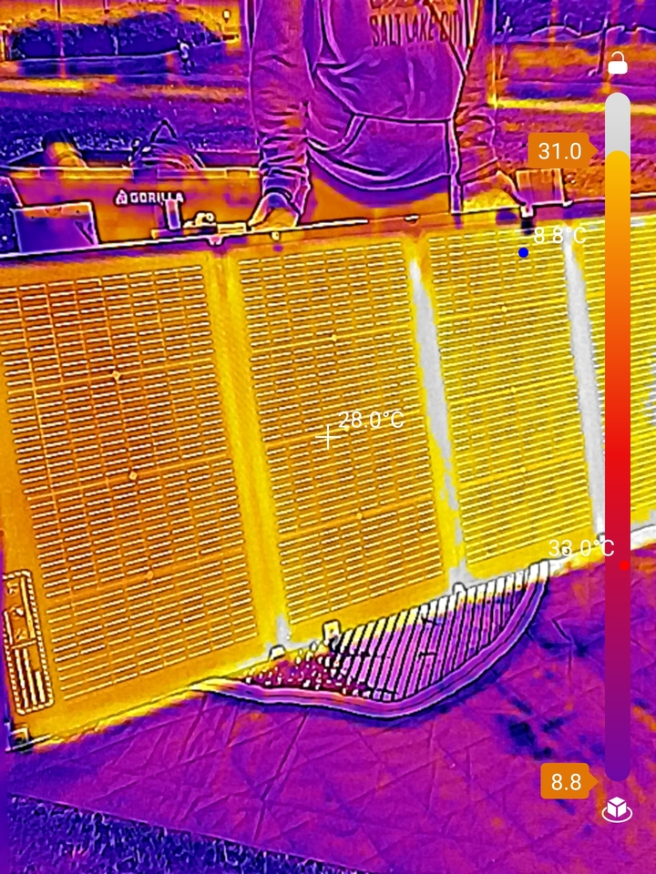
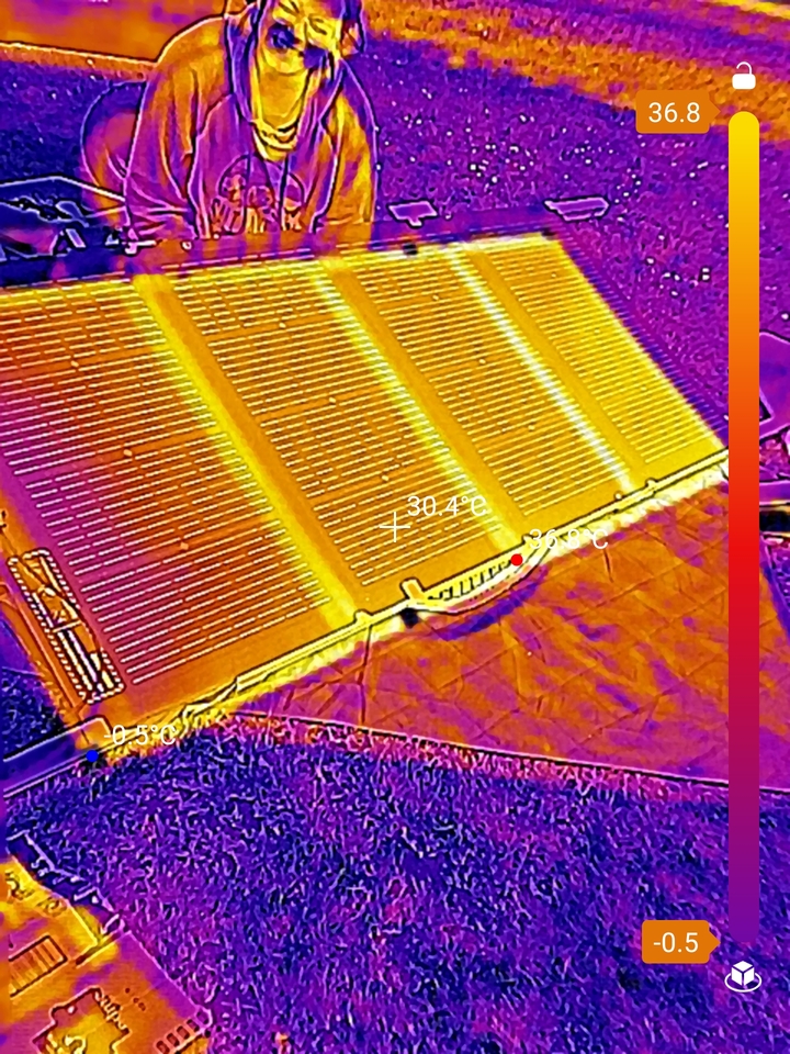
- TOPDON TC001 Thermal Camera: thermal imaging of the panel during testing
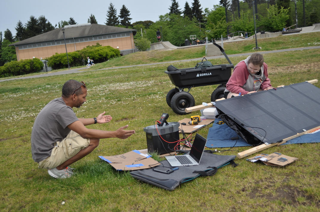
We ran two separate experiments: one testing power output at varying incident angles, and one testing power output when sub-panels were progressively blocked. Data was collected across three days: May 4, May 5, and May 9, 2026.
Voltage stayed remarkably stable across all conditions (16.4–18.1V), while power changed significantly. Using P = IV, we could infer that current was above 10A in many settings, beyond the range of any digital multimeter we had access to. So we couldn't get direct current readings. Instead we relied on the EcoFlow DELTA 2 Max power station's built-in display for power readings, and used the multimeter only for voltage verification.
We could theoretically calculate current using P = V²/R or P = I²R, but there's an unknown here: the power station itself may have internal losses between the panel and the display reading. We don't know the internal circuitry well enough to account for that precisely. Since we used the same measurement setup for all trials, the readings are consistent relative to each other, it's more of a calibrated point of reference than an absolute measurement. We're confident the displayed power was very close to actual, but we flag it as a source of uncertainty.
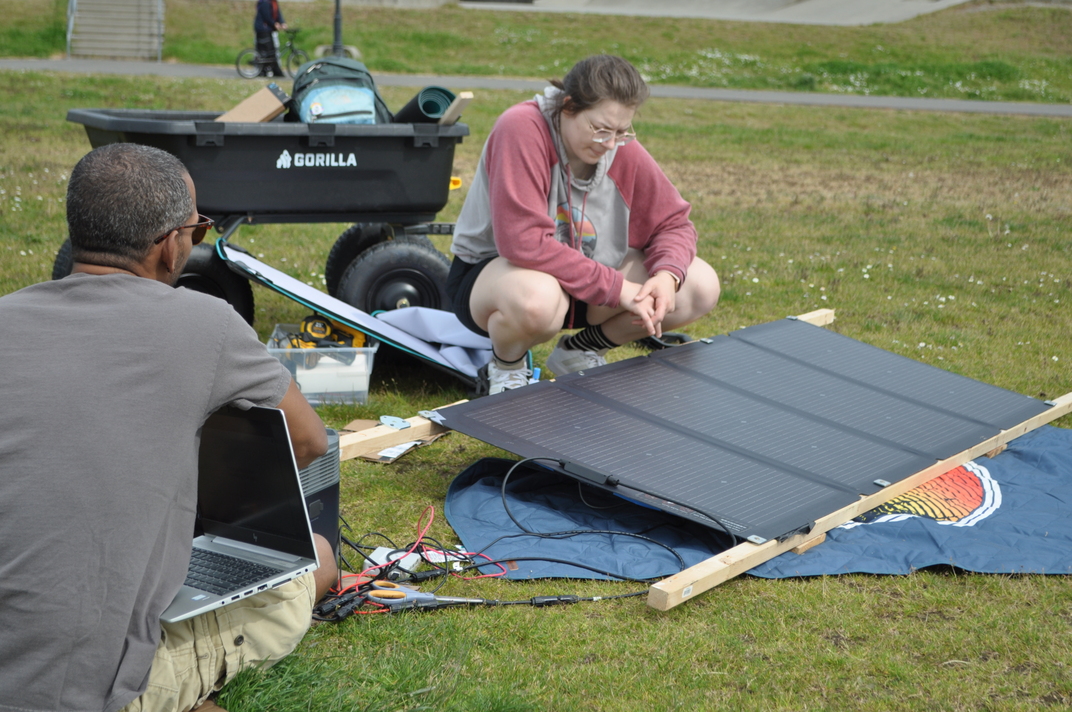
Six trials across three days. May 4 was a single run in the morning with 30° increments. May 5 had two back-to-back runs in the evening. May 9 had three runs in the afternoon, with improved angle stability thanks to a wooden frame Jose built to hold the panel steady. The first day's angle readings could be off by up to ±10° due to manually holding the panel.
| Trial | Date & Time | Angle range | P at 0° | P at max angle | Conditions |
|---|---|---|---|---|---|
| May 4 T1 | 10:24 AM | 0° → 150.1° | 182 W | 0 W @ 150° | Sunny, hand-held |
| May 5 T1 | 5:13 PM | 0° → 90.4° | 167 W | 0 W @ 90° | Evening, sun setting |
| May 5 T2 | 5:16 PM | 0° → 90.0° | 158 W | 0 W @ 90° | Evening, sun setting |
| May 9 T1 | 2:35 PM | 0° → 105.0° | 103 W | 29 W @ 105° | Overcast, cloudy |
| May 9 T2 | 2:53 PM | 0° → 120.2° | 138 W | 0 W @ 120° | Overcast, cloudy |
| May 9 T3 | 3:04 PM | 0° → 120.0° | 121 W | 0 W @ 120° | Overcast, cloudy |
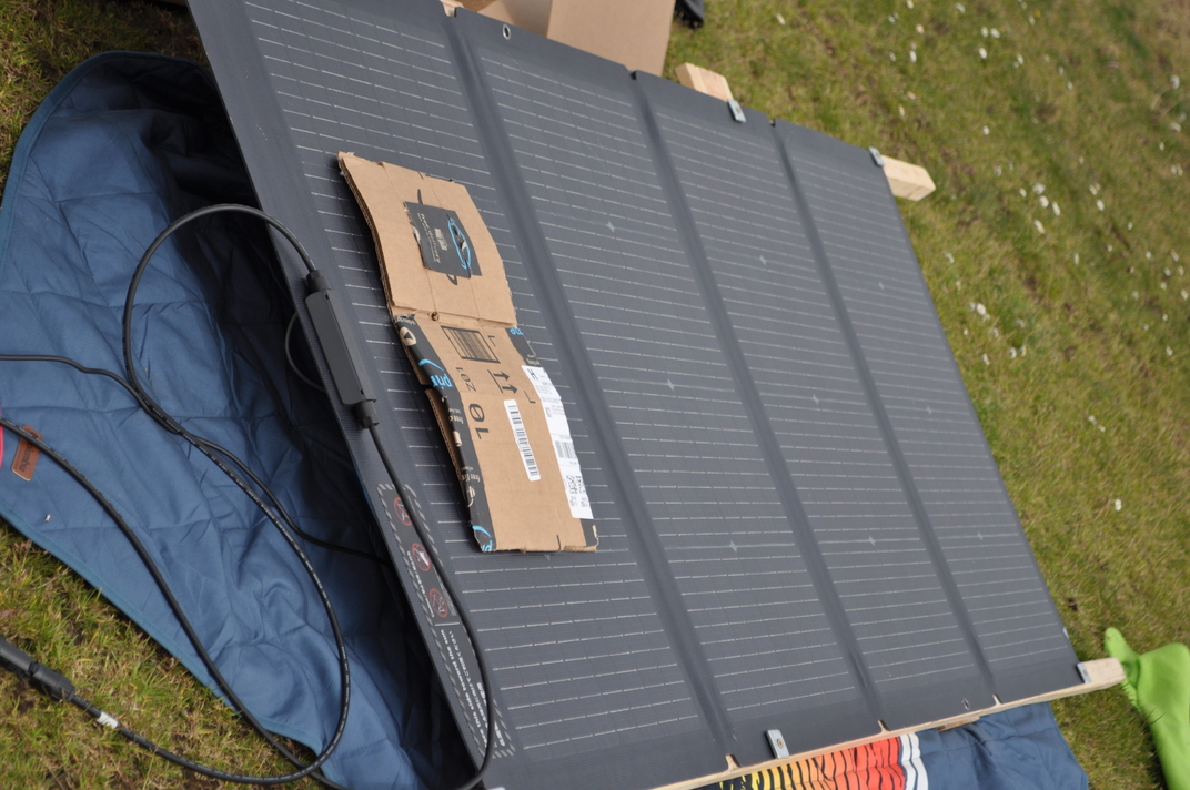
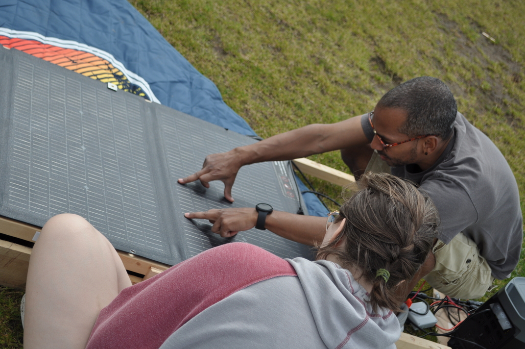
On May 9, after the angle trials, we tested what happened when sub-panels were progressively blocked. We used a Columbia blanket, cardboard, and Amanda's 3 fingers (whatever was nearby) to block portions of the panel. The big surprise: blocking just 1/8 of a single sub-panel had the same effect as blocking the whole sub-panel.
The blocking data drops in discrete 25% jumps, one per blocked sub-panel, rather than smoothly. We initially expected a linear relationship but what we saw was more like an on/off switch per sub-panel: once any portion of a sub-panel is covered, that branch goes to zero. Adding it up across sub-panels gives you a step pattern. It wasn't a model we had covered in class, but it described the data better than a line.
| Blocking | Object used | Power output | % of baseline |
|---|---|---|---|
| 0 sub-panels | Nothing | ~100 W | 100% |
| 3 fingers (1 sub-panel) | Fingers | 103 W | ~94% * |
| 1/8 of 1 sub-panel | Cardboard box | ~75 W | ~75% |
| Bottom 25% of panel | Columbia blanket | ~75 W | ~75% |
| 2 sub-panels | Blanket | ~50 W | ~50% |
| 3 sub-panels | Blanket | ~25 W | ~25% |
| 4 sub-panels (full) | Blanket | 0 W | 0% |
The best fit for the incident angle data is proportional to the square: P = Aθ², where A is a coefficient, θ is the incident angle, and P is power output. It doesn't look like a typical proportional squared curve (which usually starts at the origin) because we measured by incidence rather than by panel surface angle, so the curve is flipped, with power decreasing as angle increases and a negative slope.
This is easier to see in the normalized graph, where all trials are scaled so 0° = 100%. The curves aren't identical but follow the same pattern: a negative, curving cascade reaching 0% power somewhere between 90° and 150° depending on the day.
We expected power to hit zero at 90° incidence. On May 5, that's exactly what happened. But on May 4 and May 9, the panel kept generating past 90°. We think this is because ambient light (reflected and refracted off surrounding surfaces, clouds, and nearby objects) was significant enough to keep some current flowing even when the panel wasn't directly facing the sun. On the overcast May 9 day especially, cloud formations were acting like a diffuse light source from multiple directions.
No matter the angle, voltage stayed in the 16.4–18.1V range across all trials while power changed dramatically. Since power = voltage × current (P = IV), if voltage stays the same and power drops, current must be dropping too. The EcoFlow power station was doing something smart in the background to keep voltage stable, essentially finding the sweet spot automatically so we were always getting the most out of the panel.
Voltage actually crept up slightly at steeper angles when less light was hitting the panel. We weren't sure why at first, but it makes sense: with less current flowing, there's less electrical resistance fighting it, so voltage has room to rise a little. You can see it in the data: 16.4V at 0° on May 4, climbing to 17.2V by 150°.
This one caught us off guard. When we blocked 1/8 of one sub-panel with a small flattened cardboard box, the entire sub-panel went to zero. Same drop as blocking the whole sub-panel. We tried it again. Same result. Three fingers across one sub-panel: same 25% drop as a full block.
We're not sure why the fingers behaved differently. They might not be fully opaque, they might not seal the edges of the sub-panel completely, or the cells in that region could be arranged differently than we assumed. We only tested it a couple of times so we can't say for sure. It's one of our open questions.
The conclusion: each sub-panel's cells are wired in series internally. Block any cell in the string and the whole string is cut off. Current can't flow in or out. The other three sub-panels (in parallel) kept running normally, so we lost exactly 25% per blocked sub-panel. The blocking data drops in discrete 25% jumps, one per blocked sub-panel, rather than smoothly. Adding it up across sub-panels gives you a step pattern. It wasn't a model we had covered in class, but it described the data better than a line.
We were upfront with ourselves about where error could come in:
- Angle measurement: Manually holding a flexible panel at a precise angle is hard. May 4 readings could be off by up to ±10°. The wooden frame Jose built for May 9 helped a lot but it was still a manual hold.
- Finding true 0°: The panel spec sheet says it has a 10° window of maximum power generation around normal — so we couldn't pinpoint the exact normal precisely.
- Blocking material: The material we used in our first blocking experiment wasn't fully opaque, which skewed those readings. We caught this and used better materials later.
- Weather: Cloud cover on May 9 was constantly changing, which meant lux was fluctuating during measurements. We tried to complete each trial within 15 minutes to minimize this.
- Current: We couldn't measure current directly (it exceeded our multimeter's range). We inferred it from P = IV using the EcoFlow's power readings, which may have minor internal losses we couldn't account for.
- Panel orientation: The panel is bifacial — it generates power from both sides. We covered the back with a taped black garbage bag to isolate the front side only. We're confident it stayed covered throughout testing, but it was taped on rather than fixed, so there's a small chance it shifted or became partially exposed without us noticing. We don't believe this affected our readings, but we flag it as a possibility.
Baseline power varied significantly: 182W on May 4, 158–167W on May 5, 103–138W on May 9. That's the sun and conditions, not the panel. Once we normalized each trial to its own 0° reading, the curve shapes aligned much more consistently, confirming the angular behavior is real and repeatable even when absolute power levels differ.
We used a TOPDON TC001 thermal camera to image the panel during testing. The thermal images make the shading behavior immediately obvious: a blocked sub-panel shows up as a cold zone while the other three branches stay warm and active. It's one thing to see it in the numbers, another to see it in color.
When we fit a 2nd-degree polynomial to our data and started looking for why the curve had that particular shape, we came across Lambert's cosine law. It describes how the power received by a surface varies with the cosine of the angle between the light source and the surface normal, and it matched our data surprisingly well. We weren't testing for it going in, but the data led us there.
The polynomial fit actually tracked our measurements slightly better than the pure cosine model, which makes sense. A real panel outdoors isn't a perfect Lambertian surface. There's reflectance, atmospheric scatter, ambient light from nearby surfaces, and measurement error in the angle gauge all playing a role. But the cosine relationship is clearly there underneath it all.
The shading finding ended up being just as interesting as the angle data. In a real installation, a shadow from a chimney or tree branch hitting even a small portion of one sub-panel wipes out that entire branch. That's 25% of your output gone, same as if a quarter of the panel didn't exist. That's not obvious until you see it happen.
Not everything wrapped up neatly though. The 3-finger result is still an open question: it didn't behave the way the cardboard did, and we don't have enough data to say why. Something to test another sunny day.
Voltage stayed rock solid throughout everything, which confirmed the EcoFlow's MPPT controller was continuously finding the optimal operating point as conditions changed. The electronics handled themselves. We just had to keep rotating the panel.
The experiment answered what we set out to answer, but opened up more than it closed. Here's what we still want to test:
- The day we discovered the small-shading behavior was on a super overcast day with constantly fluctuating cloud coverage. What would that data look like on a bright, sunny day?
- An eighth of a sub-panel was enough to completely shut off power from that sub-panel. How big are the cells inside? What is the maximum amount that can be shaded before losing all power from that branch?
- What would power generation look like if we placed three fingers on each sub-panel at the same time?
- The 3-finger result didn't drop 25% like the cardboard did. Something to test another sunny day.
A plain-English guide to the technical terms that kept coming up in this project. No engineering degree required.
Links we used throughout the project and that are worth reading if you want to go deeper.
U.S. Department of Energy primer on how solar cells convert sunlight into electricity. Good starting point if you want to understand what's happening inside the panel.
NOAA's solar position calculator. Enter a location and date and it tells you solar elevation and azimuth at any time of day. We used this to understand how high the sun was during our trials.
The official panel manual. Includes full spec sheet, and the 10-degree normal incidence window we referenced in our uncertainty analysis.
| Incident angle | Measured (W) | Measured (V) | Poly pred. | Poly err. |
|---|
| Rated power (STC) | 220 W ±5 W |
| Real-world max (front, 0°) | 180 W |
| Open circuit voltage Voc | 21.8 V |
| Max power voltage Vmp | 18.4 V |
| Short circuit current Isc (STC) | 13.0 A |
| Max power current Imp (STC) | 12.0 A |
| Operating Imp (180W ÷ 18.4V) | ~9.78 A total |
| Per sub-panel operating Imp | ~2.45 A each |
| Power temp. coeff. | -0.39 %/K |